This notebook demonstrates how to move between a probability density function PDF and cumulative density function CDF . If one has a PDF, a CDF may be derived from integrating over the PDF; if one has a CDF, the PDF may be derived from taking the derivative over the CDF.
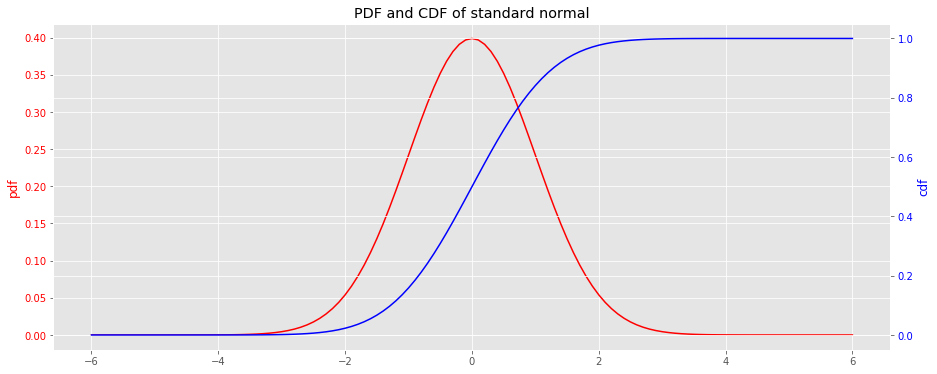
Here, we visualize the PDF and CDF for the standard normal distribution. The functions scipy.stats.norm.pdf and scipy.stats.norm.cdf will be used to generate the curves and data.
import matplotlib.pyplot as plt import numpy as np import pandas as pd from scipy.stats import norm import warnings plt.style.use('ggplot') np.random.seed(37) warnings.filterwarnings('ignore')
x = np.arange(-6, 6.1, 0.1) y_pdf = norm.pdf(x) y_cdf = norm.cdf(x) fig, ax = plt.subplots(figsize=(15, 6)) ax = [ax, ax.twinx()] _ = ax[0].plot(x, y_pdf, label='pdf', color='r') _ = ax[1].plot(x, y_cdf, label='cdf', color='b') _ = ax[0].tick_params(axis='y', labelcolor='r') _ = ax[1].tick_params(axis='y', labelcolor='b') _ = ax[0].set_ylabel('pdf', color='r') _ = ax[1].set_ylabel('cdf', color='b') _ = ax[0].set_title('PDF and CDF of standard normal')
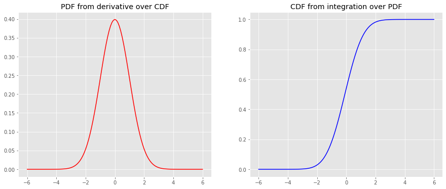
We will use scipy.misc.derivative and scipy.integrate.quad to take the derivative of the CDF to get the PDF and to integrate the PDF to get the CDF, respectively.
from scipy.misc import derivative from scipy.integrate import quad y_cdf = np.array([tup[0] for tup in [quad(norm.pdf, a, b) for a, b in [(a, b) for a, b in zip(x, x[1:len(x)])]]] + [0]).cumsum() y_pdf = derivative(norm.cdf, x, dx=1e-6) fig, ax = plt.subplots(1, 2, figsize=(15, 6)) _ = ax[0].plot(x, y_pdf, color='r') _ = ax[1].plot(x, y_cdf, color='b') _ = ax[0].set_title('PDF from derivative over CDF') _ = ax[1].set_title('CDF from integration over PDF')
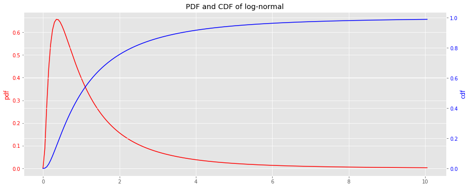
from scipy.stats import lognorm lognorm_pdf = lambda x: lognorm.pdf(x, 1) lognorm_cdf = lambda x: lognorm.cdf(x, 1) x = np.arange(0, 10.1, 0.05) y_pdf = lognorm_pdf(x) y_cdf = lognorm_cdf(x) fig, ax = plt.subplots(figsize=(15, 6)) ax = [ax, ax.twinx()] _ = ax[0].plot(x, y_pdf, label='pdf', color='r') _ = ax[1].plot(x, y_cdf, label='cdf', color='b') _ = ax[0].tick_params(axis='y', labelcolor='r') _ = ax[1].tick_params(axis='y', labelcolor='b') _ = ax[0].set_ylabel('pdf', color='r') _ = ax[1].set_ylabel('cdf', color='b') _ = ax[0].set_title('PDF and CDF of log-normal')
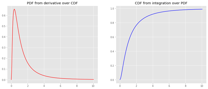
y_cdf = np.array([tup[0] for tup in [quad(lognorm_pdf, a, b) for a, b in [(a, b) for a, b in zip(x, x[1:len(x)])]]] + [0]).cumsum() y_pdf = derivative(lognorm_cdf, x, dx=1e-6) fig, ax = plt.subplots(1, 2, figsize=(15, 6)) _ = ax[0].plot(x, y_pdf, color='r') _ = ax[1].plot(x, y_cdf, color='b') _ = ax[0].set_title('PDF from derivative over CDF') _ = ax[1].set_title('CDF from integration over PDF')
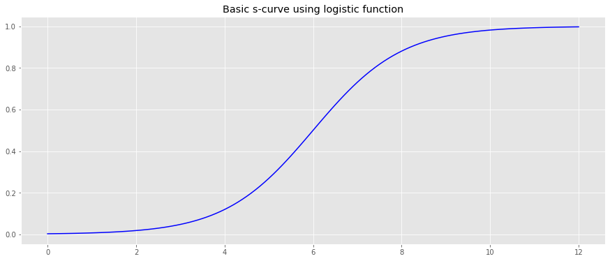
We will generate an arbitrary CDF using the logistic function.
logistic = lambda x, L=1, x_0=0, k=1: L / (1 + np.exp(-k * (x - x_0))) x = np.arange(-6, 6.1, 0.1) y = logistic(x) x = x + 6.0 fig, ax = plt.subplots(figsize=(15, 6)) _ = ax.plot(x, y, color='b') _ = ax.set_title('Basic s-curve using logistic function')
The parameters, \(L\) , \(x_0\) and \(k\) , for the logistic function will be learned.
from scipy.optimize import curve_fit L_estimate = y.max() x_0_estimate = np.median(x) k_estimate = 1.0 p_0 = [L_estimate, x_0_estimate, k_estimate] popt, pcov = curve_fit(logistic, x, y, p_0, method='dogbox') L, x_0, k = popt[0], popt[1], popt[2]
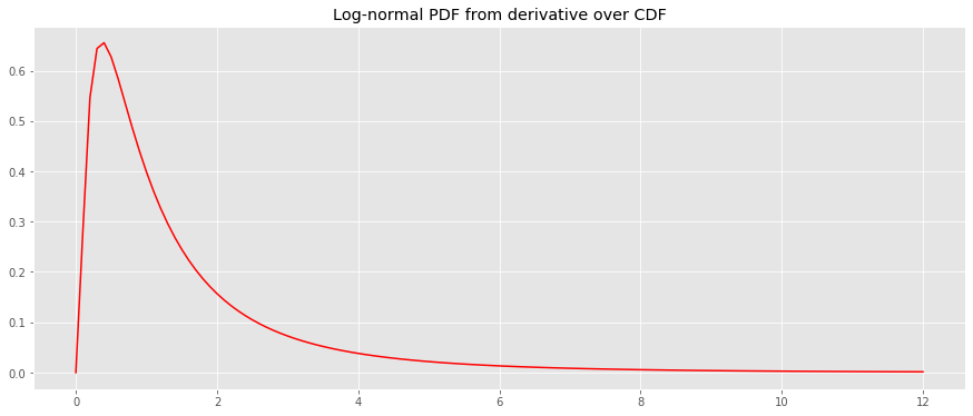
Assuming the PDF is log-normal, we will take the derivative of the CDF to estimate the PDF.
logistic = lambda x, L=L, x_0=x_0, k=k: L / (1 + np.exp(-k * (x - x_0))) y_pdf = derivative(lognorm_cdf, x, dx=1e-6) fig, ax = plt.subplots(figsize=(15, 6)) _ = ax.plot(x, y_pdf, color='r') _ = ax.set_title('Log-normal PDF from derivative over CDF')
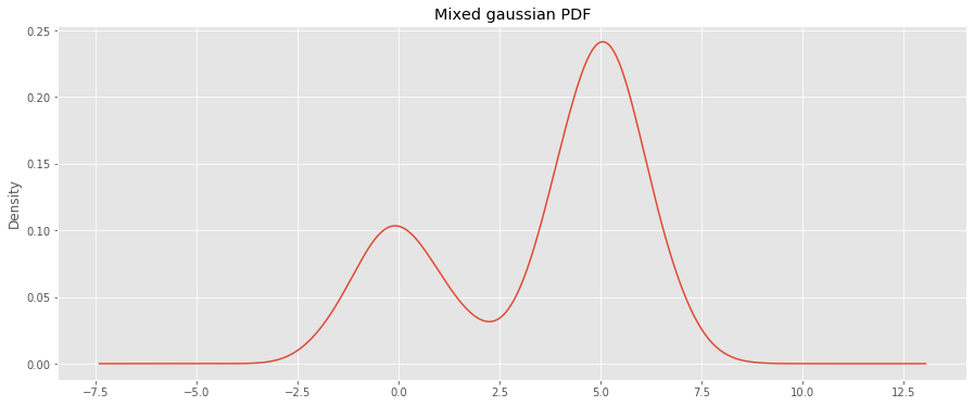
We will generate a guassian-mixture (GM) PDF and derive the CDF using integration.
N = 1000 X = np.concatenate((np.random.normal(0, 1, int(0.3 * N)), np.random.normal(5, 1, int(0.7 * N))))
s = pd.Series(X) fig, ax = plt.subplots(figsize=(15, 6)) _ = s.plot(kind='kde', bw_method='scott', ax=ax) _ = ax.set_title('Mixed gaussian PDF')
We then use a kernel density estimator to learn the PDF.
from sklearn.neighbors import KernelDensity kde = KernelDensity(kernel='gaussian', bandwidth=0.75).fit(X[:, np.newaxis]) gmm_pdf = lambda x: np.exp(kde.score(np.array([x]).reshape(-1, 1)))
Finally, the CDF of the PDF will be estimated using integration.
%%time x = np.arange(-5, 10.1, 0.1) y_cdf = np.array([tup[0] for tup in [quad(gmm_pdf, a, b) for a, b in [(a, b) for a, b in zip(x, x[1:len(x)])]]] + [0]).cumsum()
CPU times: user 522 ms, sys: 0 ns, total: 522 ms Wall time: 548 ms
fig, ax = plt.subplots(figsize=(15, 6)) _ = ax.plot(x, y_cdf, color='b') _ = ax.set_title('CDF from integration over gaussian-mixture PDF')

© Copyright 2019, One-Off Coder. Last updated on Apr 03, 2024, 4:35:01 PM.